


Multivariable calculus (Calculus 3) extends derivatives and integrals to functions of several variables, such as ( z = f(x, y) ). Its main tools are vectors (including dot products and vector projection), partial derivatives, the gradient ( nabla f ), double and triple integrals, and vector calculus with Green’s, Stokes’ and the divergence theorems.
Multivariable calculus (also called Calculus 3 or multidimensional calculus) extends derivatives and integrals from functions of one variable, ( y = f(x) ), to functions of several variables, such as ( z = f(x, y) ) or ( T = f(x, y, z) ). Instead of curves, you work with surfaces, solids and fields.
Most of the ideas carry over from single-variable calculus. A derivative is still a rate of change, but now you have to say in which direction. An integral still adds up small pieces, but the pieces are tiny squares or cubes instead of thin strips.
What multivariable calculus covers
| Topic | Single-variable version | Multivariable version |
|---|---|---|
| Functions | ( y = f(x) ), a curve | ( z = f(x, y) ), a surface |
| Space | the number line | vectors in 2D and 3D |
| Derivatives | ( f'(x) ) | partial derivatives ( f_x, f_y ) and the gradient ( nabla f ) |
| Optimization | ( f'(x) = 0 ) | ( nabla f = mathbf{0} ), second derivative test, Lagrange multipliers |
| Integrals | ( int_a^b f(x),dx ) | double and triple integrals |
| Fundamental theorem | ( int_a^b F'(x),dx = F(b) – F(a) ) | Green’s, Stokes’ and the divergence theorems |
Vectors
A vector has a size and a direction, written ( mathbf{v} = langle v_1, v_2, v_3 rangle ). Its length is ( |mathbf{v}| = sqrt{v_1^2 + v_2^2 + v_3^2} ), the three-dimensional distance formula.
Dot product
$$mathbf{a}cdotmathbf{b} = a_1b_1 + a_2b_2 + a_3b_3 = |mathbf{a}||mathbf{b}|costheta$$
The dot product is zero exactly when the vectors are perpendicular. It also finds the angle between two vectors.
Vector projection
The projection of ( mathbf{b} ) onto ( mathbf{a} ) is the shadow ( mathbf{b} ) casts along ( mathbf{a} ):
$$text{proj}_{mathbf{a}}mathbf{b} = frac{mathbf{a}cdotmathbf{b}}{|mathbf{a}|^2},mathbf{a}$$
Example 1. Project ( mathbf{b} = langle 2, 3 rangle ) onto ( mathbf{a} = langle 4, 0 rangle ). Then ( mathbf{a}cdotmathbf{b} = 8 ) and ( |mathbf{a}|^2 = 16 ), so ( text{proj}_{mathbf{a}}mathbf{b} = frac{8}{16}langle 4, 0 rangle = langle 2, 0 rangle ): the horizontal part of b, as you’d expect. Projections split a force into the part along a ramp and the part pushing into it, and they compute work done by a force.
Cross product
In 3D, ( mathbf{a}timesmathbf{b} ) is a vector perpendicular to both, with length equal to the area of the parallelogram they span. It gives normal vectors to planes and torque in physics.
Functions of several variables
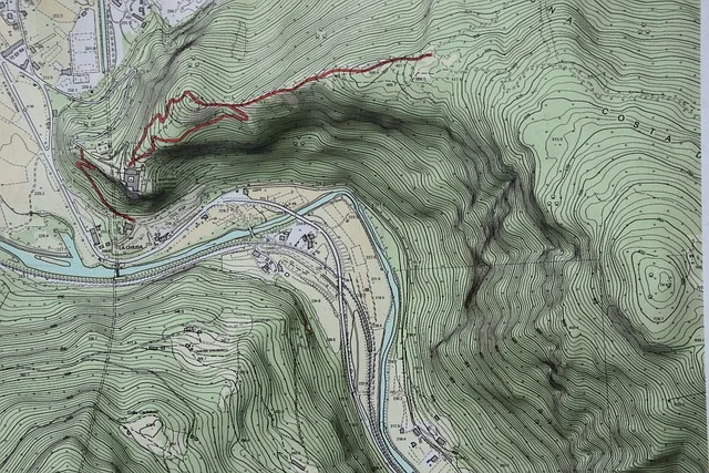
( f(x, y) = x^2 + y^2 ) assigns a height to every point of the plane; its graph is a bowl (a paraboloid). Level curves, where ( f(x, y) = c ), are the contour lines on a map: here, circles centered at the origin.
Partial derivatives
A partial derivative measures change in one variable while holding the others fixed. For ( f_x ), treat y as a constant and differentiate with respect to x.

Example 2. For ( f(x, y) = x^2y + 3y^2 ):
$$f_x = 2xy, qquad f_y = x^2 + 6y$$
At ( (1, 2) ), ( f_x = 4 ) and ( f_y = 13 ): moving in the y direction, the surface rises more than three times as steeply as in the x direction.
The partial derivatives guide covers second partials and the chain rule, and the partial derivative calculator handles any function.
The gradient and directional derivatives
The gradient collects the partial derivatives into a vector:
$$nabla f = langle f_x, f_y rangle$$
It points in the direction of steepest increase, and its length is the steepest rate. The rate of change in any unit direction ( mathbf{u} ) is the directional derivative ( D_{mathbf{u}}f = nabla fcdotmathbf{u} ), a dot product.
Example 3. For ( f = x^2 + y^2 ) at ( (3, 4) ), ( nabla f = langle 6, 8 rangle ) with length 10. Heading in the x direction, ( mathbf{u} = langle 1, 0 rangle ), the rate is only 6. See the gradient and directional derivative guide and the gradient calculator.
Optimization
Critical points are where ( nabla f = mathbf{0} ). The second derivative test uses ( D = f_{xx}f_{yy} – f_{xy}^2 ): if ( D > 0 ) and ( f_{xx} > 0 ) it’s a minimum, if ( D > 0 ) and ( f_{xx} < 0 ) a maximum, and if ( D < 0 ) a saddle point. For maximizing with a constraint, such as the largest box with a fixed surface area, Lagrange multipliers solve ( nabla f = lambdanabla g ).

Double and triple integrals
A double integral adds ( f(x, y) ) over a region, giving the volume under a surface:
$$iint_R f(x, y),dA = int_a^b int_c^d f(x, y),dy,dx$$
You evaluate it as two ordinary integrals, inside first.
Example 4. Over ( R = [0, 1] times [0, 2] ):
$$int_0^1 int_0^2 (x + y),dy,dx = int_0^1 left[ xy + tfrac12y^2 right]_0^2 dx = int_0^1 (2x + 2),dx = 3$$
Dividing by the area 2 gives the average value 1.5. See double integrals and the double integral calculator. Triple integrals do the same over solids, and polar, cylindrical and spherical coordinates simplify round regions.
Vector calculus
The final part of the course studies vector fields (wind, fluid flow, electric fields) with line integrals, surface integrals, divergence and curl. Its three big theorems, Green’s, Stokes’ and the divergence theorem, are all versions of the Fundamental Theorem of Calculus: an integral of a derivative over a region equals a sum over its boundary.
Is multivariable calculus hard?
It’s mostly familiar techniques applied more than once. The new challenge is visualizing in three dimensions. Students who are comfortable with single-variable derivatives and integrals, plus a little vector algebra, usually do well. Calculus 3 is often considered easier than Calculus 2.
Common mistakes
- Forgetting to hold variables constant. In ( frac{partial}{partial x}(x^2y) ), y is a constant, so the answer is ( 2xy ), not ( 2xy + x^2y’ ).
- Using a non-unit direction. Normalize ( mathbf{u} ) before computing ( nabla fcdotmathbf{u} ).
- Mixing up integration order and limits. The inner integral’s limits go with the inner variable.
- Confusing the dot and cross products. Dot gives a number; cross gives a vector, and only in 3D.
Practice problems
- Find ( |langle 2, -1, 2 rangle| ).
- Find ( text{proj}_{mathbf{a}}mathbf{b} ) for ( mathbf{a} = langle 1, 1 rangle ), ( mathbf{b} = langle 3, 5 rangle ).
- Find ( f_x ) and ( f_y ) for ( f(x, y) = x^3 + 2xy^2 ).
- Find ( nabla f ) at ( (1, 1) ) for ( f(x, y) = xy^2 ).
- Evaluate ( int_0^2 int_0^1 6xy,dy,dx ).
Answers: (1) 3; (2) ( langle 4, 4 rangle ); (3) ( f_x = 3x^2 + 2y^2 ), ( f_y = 4xy ); (4) ( langle 1, 2 rangle ); (5) 6.
FAQ
What is multivariable calculus?
Calculus for functions of more than one variable: partial derivatives, gradients, multiple integrals and vector calculus.
Is multivariable calculus the same as Calculus 3?
In most US universities, yes. Some schools call it vector calculus or multivariable and vector calculus.
What do I need before multivariable calculus?
Single-variable differentiation and integration (Calculus 1 and 2). Some vector algebra helps, but it’s taught at the start of the course.
What is multivariable calculus used for?
Physics and engineering (fields, fluid flow, electromagnetism), economics (optimization with several inputs), computer graphics, and machine learning, where training a model means following the gradient downhill.
What is the difference between a derivative and a partial derivative?
An ordinary derivative applies to a function of one variable. A partial derivative applies to a function of several, differentiating in one variable while the others are held constant.
Further reading
- Calculus III (Paul’s Online Math Notes) — a complete free course covering vectors, partial derivatives, multiple integrals and vector calculus.
- Multivariable calculus (Wikipedia) — an overview of the subject, its main theorems and applications.
Calculators for this topic
Keep learning
Double Integrals: How to Evaluate Them Step by Step
Evaluate double integrals as iterated integrals, switch the order of integration, and use polar coordinates. Step-by-step worked examples.

Gradient and Directional Derivative: Formulas and Examples
The gradient ∇f collects partial derivatives; the directional derivative D_u f = ∇f · u gives the slope in any direction. Worked example and geometric meaning.