Intermediate Value Theorem (IVT): Statement and Examples

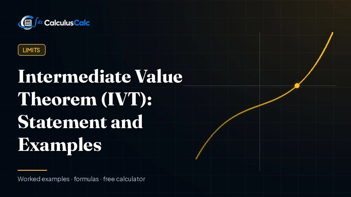
The Intermediate Value Theorem (IVT) says: if ( f ) is continuous on the closed interval ( [a, b] ) and ( N ) is any number between ( f(a) ) and ( f(b) ), then there is at least one ( c ) in ( (a, b) ) with ( f(c) = N ). Its most common use: if a continuous function changes sign on ( [a, b] ), it has a root in between.

The IVT turns an intuitive fact (you can’t get from one side of a line to the other without crossing it) into a precise tool. It guarantees that solutions exist even when you can’t find them with algebra, and it’s the reason numerical root-finding methods work.

The theorem

Intermediate Value Theorem. Suppose

1. ( f ) is continuous on ( [a, b] ), and
2. ( N ) is any number strictly between ( f(a) ) and ( f(b) ).

Then there is at least one number ( c ) with ( a < c < b ) and ( f(c) = N ).

Root version (Bolzano’s theorem). If ( f ) is continuous on ( [a, b] ) and ( f(a) ) and ( f(b) ) have opposite signs, then ( f(c) = 0 ) for some ( c ) in ( (a, b) ).

What it means geometrically

Draw the horizontal line ( y = N ). The graph starts on one side of it at ( x = a ) and ends on the other side at ( x = b ). A continuous graph can be drawn without lifting your pen, so it has to cross the line somewhere.

Everyday version: if the temperature was 10°C at 6 am and 20°C at noon, then at some moment in between it was exactly 15°C.

How to use the IVT

1. Check continuity on the closed interval. Polynomials, ( sin x ), ( cos x ) and ( e^x ) are continuous everywhere; rational functions are continuous except where the denominator is zero.
2. Evaluate ( f(a) ) and ( f(b) ).
3. Check that ( N ) lies between them (for roots, that the signs differ).
4. Conclude that some ( c ) in ( (a, b) ) has ( f(c) = N ). The IVT says that ( c ) exists, not where it is.

Example 1: a root of a cubic

Show that ( x^3 + x – 1 = 0 ) has a solution between 0 and 1.

( f(x) = x^3 + x – 1 ) is a polynomial, so it’s continuous on ( [0, 1] ). Then ( f(0) = -1 < 0 ) and ( f(1) = 1 > 0 ). Since 0 is between ( -1 ) and ( 1 ), the IVT guarantees a ( c ) in ( (0, 1) ) with ( f(c) = 0 ).

(In fact ( f'(x) = 3x^2 + 1 > 0 ), so ( f ) is increasing and this is the only real root, about ( c approx 0.6823 ). The uniqueness argument uses the Mean Value Theorem, not the IVT.)

Example 2: an equation with trig

Show that ( cos x = x ) has a solution.

Let ( g(x) = cos x – x ), continuous everywhere. ( g(0) = 1 > 0 ) and ( g(1) = cos 1 – 1 approx -0.4597 < 0 ). By the IVT there’s a ( c ) in ( (0, 1) ) with ( cos c = c ). It’s about ( 0.7391 ), but no algebraic formula gives it.

Example 3: hitting a value other than zero

Show that ( f(x) = x^2 + 2x ) takes the value 5 somewhere in ( [1, 2] ).

( f(1) = 3 ) and ( f(2) = 8 ). Since ( 3 < 5 < 8 ) and ( f ) is continuous, some ( c ) in ( (1, 2) ) has ( f(c) = 5 ). Here we can solve it: ( c^2 + 2c – 5 = 0 ) gives ( c = -1 + sqrt6 approx 1.449 ) (see the quadratic formula).

When the IVT does not apply

Continuity is essential. Consider ( f(x) = frac1x ) on ( [-1, 1] ): ( f(-1) = -1 ) and ( f(1) = 1 ) have opposite signs, but ( frac1x ) is never zero. The IVT fails because ( f ) isn’t continuous at ( x = 0 ), where the graph jumps from ( -infty ) to ( +infty ).

Likewise, a step function that jumps from 0 to 1 never takes the value ( frac12 ).

Also note the IVT only works one way. If ( f(a) ) and ( f(b) ) have the same sign, the function might still have roots in between (for example ( x^2 – frac14 ) on ( [-1, 1] )); the IVT simply doesn’t tell you.

Finding the root: the bisection method

The IVT suggests an algorithm. Keep halving the interval and keep the half where the sign changes:

Step	Interval	Midpoint ( m )	( f(m) ) for ( x^3 + x – 1 )	Keep
1	( [0, 1] )	0.5	( -0.375 )	( [0.5, 1] )
2	( [0.5, 1] )	0.75	( 0.1719 )	( [0.5, 0.75] )
3	( [0.5, 0.75] )	0.625	( -0.1309 )	( [0.625, 0.75] )
4	( [0.625, 0.75] )	0.6875	( 0.0125 )	( [0.625, 0.6875] )

Each step halves the uncertainty, closing in on ( c approx 0.6823 ). Newton’s method converges much faster once you’re close; try it in the Newton’s method calculator.

See it on a graph

Plot ( x^3 + x – 1 ) and look for where it crosses the x-axis between 0 and 1. Change the function to <code>cos(x) – x</code> to see Example 2.

Why the IVT is true

The full proof relies on the completeness of the real numbers (every bounded set has a least upper bound). Sketch for the root version with ( f(a) < 0 < f(b) ): let ( c ) be the least upper bound of the set of points in ( [a, b] ) where ( f < 0 ). If ( f(c) < 0 ), continuity would make ( f ) negative a little to the right of ( c ), contradicting that ( c ) is an upper bound; if ( f(c) > 0 ), it would be positive a little to the left, so a smaller upper bound would exist. Hence ( f(c) = 0 ). On the rational numbers alone the theorem fails: ( x^2 – 2 ) changes sign on ( [1, 2] ) but has no rational root.

IVT, EVT and MVT compared

Theorem	Needs	Guarantees
Intermediate Value Theorem	( f ) continuous on ( [a, b] )	( f ) takes every value between ( f(a) ) and ( f(b) )
Extreme Value Theorem	( f ) continuous on ( [a, b] )	( f ) has a maximum and a minimum on ( [a, b] )
Mean Value Theorem	continuous on ( [a, b] ), differentiable on ( (a, b) )	some ( f'(c) ) equals the average slope

The Extreme Value Theorem is what makes the closed-interval method in critical points work; the Mean Value Theorem is covered in its own guide. For more on continuity and limits, see calculus concepts.

Common mistakes

• Skipping the continuity check. Graders expect you to state it explicitly.
• Claiming to find ( c ). The IVT proves existence, not location.
• Claiming uniqueness. There may be several values of ( c ).
• Using an open interval. The theorem needs continuity on the closed interval ( [a, b] ).

Practice problems

1. Show that ( x^5 – 3x + 1 = 0 ) has a root in ( (0, 1) ).
2. Does the IVT guarantee a root of ( x^2 – 4 ) in ( [0, 1] )? Explain.
3. Show that ( e^x = 3 – x ) has a solution in ( (0, 1) ).
4. Can the IVT be used for ( f(x) = tan x ) on ( [0, pi] )? Why or why not?
5. Use two steps of bisection on ( x^2 – 2 ) over ( [1, 2] ). What interval contains ( sqrt2 )?

Answers: (1) ( f(0) = 1 > 0 ), ( f(1) = -1 < 0 ), and ( f ) is a continuous polynomial, so yes. (2) No: ( f(0) = -4 ) and ( f(1) = -3 ) have the same sign, so the IVT says nothing (and in fact there’s no root there). (3) Let ( g(x) = e^x + x – 3 ): ( g(0) = -2 ), ( g(1) = e – 2 approx 0.718 ), and ( g ) is continuous. (4) No: ( tan x ) is not continuous at ( frac{pi}{2} ). (5) ( [1.25, 1.5] ).

FAQ

What does the Intermediate Value Theorem say?

A continuous function on ( [a, b] ) takes every value between ( f(a) ) and ( f(b) ) at least once.

How do you use the IVT to show a root exists?

Show the function is continuous on ( [a, b] ), then show ( f(a) ) and ( f(b) ) have opposite signs. The IVT then guarantees a root between ( a ) and ( b ).

Why does the function have to be continuous?

Without continuity the graph can jump over a value. ( frac1x ) goes from negative to positive on ( [-1, 1] ) but never equals 0.

Does the IVT tell you where the root is?

No. It only guarantees existence. Use bisection, Newton’s method or a graph to locate it.

What is the difference between the IVT and the MVT?

The IVT is about function values (heights) and needs only continuity. The Mean Value Theorem is about slopes and also needs differentiability.

Further reading

• Intermediate value theorem (Wikipedia) — statement, proof, history and generalizations.
• Calculus I (Paul’s Online Math Notes) — continuity and the Intermediate Value Theorem in the Limits chapter.