Trapezoidal Rule Calculator (with Table and Error)

This trapezoidal rule calculator approximates a definite integral ( int_a^b f(x),dx ) by splitting the area under the curve into n trapezoids. It shows ( Delta x ), a full table of the points ( x_i ), the values ( f(x_i) ) and their weights, the weighted sum, the approximation ( T_n ), the exact integral and the error.

It’s free and needs no sign-up.

How to use it

1. Type the function, for example x^2, 1/x or e^(-x^2).
2. Enter the limits a and b and the number of subintervals n.
3. Press Approximate.

The table is shown for n up to 40; larger n still computes, just without the table.

Formula

With ( Delta x = frac{b – a}{n} ) and ( x_i = a + i,Delta x ):

$$T_n = frac{Delta x}{2}left[f(x_0) + 2f(x_1) + 2f(x_2) + cdots + 2f(x_{n-1}) + f(x_n)right]$$

The two endpoints get weight 1. Every interior point gets weight 2. This is because it is shared by two neighboring trapezoids. Each trapezoid has area ( frac{Delta x}{2}[f(x_{i-1}) + f(x_i)] ). Adding these gives the formula. A trapezoidal rule calculator uses this method. It is also the average of the left and right Riemann sums.

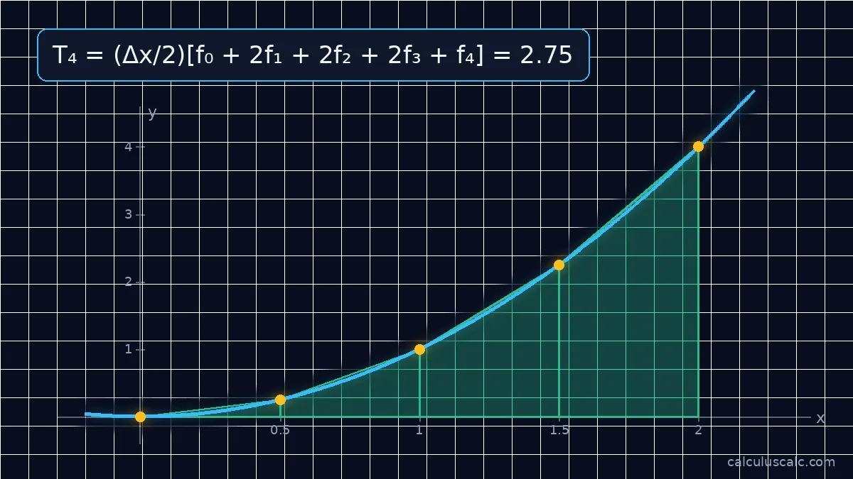
Worked example: ∫₀² x² dx with n = 4

As loaded above: ( Delta x = frac{2 – 0}{4} = frac{1}{2} ).

i	( x_i )	( f(x_i) )	Weight	Weight × f
0	0	0	1	0
1	0.5	0.25	2	0.5
2	1	1	2	2
3	1.5	2.25	2	4.5
4	2	4	1	4

The weighted sum is 11, so

$$T_4 = frac{1/2}{2} times 11 = frac{11}{4} = 2.75$$

The exact value is ( frac{8}{3} approx 2.6667 ), so the error is ( frac{1}{12} approx 0.0833 ). The trapezoids overestimate because ( x^2 ) is concave up: each straight top lies above the curve.

Worked example: distance from speed readings

A car’s speed is recorded every 2 seconds:

t (s)	0	2	4	6	8
v (m/s)	0	6	10	12	13

Distance is the integral of speed. With ( Delta t = 2 ):

$$T_4 = frac{2}{2}left[0 + 2(6 + 10 + 12) + 13right] = 69 text{ m}$$

This is where the trapezoidal rule is most useful: when you only have measurements, not a formula.

Worked example: ln 2

( int_1^2 frac{1}{x},dx = ln 2 approx 0.693147 ). With n = 4 the trapezoidal rule gives 0.697024, an error of about 0.0039. However, doubling n to 8 cuts the error to about 0.00098, roughly a quarter.

Error bound

If ( |f”(x)| le K ) on ( [a, b] ), then

$$|E_T| le frac{K(b - a)^3}{12n^2}$$

The error shrinks like ( frac{1}{n^2} ): doubling n divides the error by about 4. For ( x^2 ) on ( [0, 2] ), ( K = 2 ) and the bound is ( frac{2 cdot 8}{12 cdot 16} = frac{1}{12} ), exactly the actual error, because ( f” ) is constant.

Using a trapezoidal rule calculator versus Simpson's rule

Simpson’s rule fits parabolas, not straight lines. It is usually more accurate for the same n. Its error shrinks like ( frac{1}{n^4} ). For the ( x^2 ) example, Simpson’s rule gives the exact answer. Use a trapezoidal rule calculator when n is odd. Also use it for uneven data. Or use it for the simplest method.

Common mistakes

• Giving the endpoints weight 2. Only interior points are doubled.
• Dividing by 3 instead of 2. That’s Simpson’s rule.
• Using ( Delta x = frac{b – a}{n + 1} ). n subintervals use ( n + 1 ) points, but ( Delta x = frac{b – a}{n} ).

Step-by-step method

1. Compute ( Delta x = frac{b – a}{n} ).
2. List the points ( x_0 = a, x_1 = a + Delta x, ldots, x_n = b ).
3. Evaluate f at each point.
4. Multiply the first and last values by 1 and all the others by 2, then add.
5. Multiply the sum by ( frac{Delta x}{2} ).

Worked example: ∫₀⁴ √x dx with n = 4

( Delta x = 1 ) and the points are 0, 1, 2, 3, 4:

$$T_4 = frac{1}{2}left[0 + 2(1 + 1.4142 + 1.7321) + 2right] = frac{1}{2}(10.2925) approx 5.1463$$

The exact value is ( frac{16}{3} approx 5.3333 ). This time the rule underestimates, because ( sqrt{x} ) is concave down: the straight tops of the trapezoids lie below the curve.

Worked example: estimating π

Since ( int_0^1 frac{1}{1 + x^2},dx = arctan 1 = frac{pi}{4} ), numerical integration can estimate π. With n = 4 the trapezoidal rule gives 0.782794, so ( pi approx 4 times 0.782794 = 3.1312 ). Simpson’s rule with the same five points gives 3.141569, within 0.00003 of π.

Trapezoid vs Riemann sums

Method	For ( int_0^1 e^x,dx ), n = 4	Error
Left Riemann sum	1.5124	0.2059
Right Riemann sum	1.9420	0.2237
Trapezoidal rule	1.7272	0.0089
Simpson’s rule	1.7183	0.00004

The exact value is ( e – 1 approx 1.7183 ). The trapezoidal rule is the average of the left and right sums, which is why it is so much better than either. Try the Riemann sum calculator to compare them yourself.

Applications

Surveyors find irregular plot area from spaced measurements. Engineers integrate sensor readings (speed to distance, power to energy). Pharmacologists compute drug concentration “area under the curve”. Also, economists estimate total revenue from sampled rates. A trapezoidal rule calculator handles this tabular data directly for all these tasks.

Practice problems

1. Approximate ( int_0^2 x^3,dx ) with n = 2.
2. Approximate ( int_1^3 frac{1}{x},dx ) with n = 2.
3. A tank’s inflow rate (L/min) is 4, 7, 9, 8 and 6 at t = 0, 1, 2, 3, 4 minutes. Estimate the total inflow.

Answers: 1. ( Delta x = 1 ): ( frac{1}{2}[0 + 2(1) + 8] = 5 ) (exact 4). 2. ( Delta x = 1 ): ( frac{1}{2}[1 + 2(0.5) + 0.3333] = 1.1667 ) (exact ( ln 3 approx 1.0986 )). 3. ( frac{1}{2}[4 + 2(7 + 9 + 8) + 6] = 29 ) litres.

How fast the error falls

For ( int_0^2 x^2,dx ) the error with n = 4 is ( frac{1}{12} approx 0.0833 ); with n = 8 it is ( frac{1}{48} approx 0.0208 ), exactly a quarter, as the ( frac{1}{n^2} ) error bound predicts. As a result, to get one more correct decimal place you need about three times as many subintervals.

Related guides

• Riemann Sums
• Simpson’s Rule Calculator
• Fundamental Theorem of Calculus
• Definite Integral Calculator

Further reading

• Trapezoidal rule (Wikipedia) — derivation, error analysis and uneven grids.

FAQ

What is the trapezoidal rule?

A way to approximate a definite integral by dividing the area into trapezoids and adding their areas: ( T_n = frac{Delta x}{2}[f(x_0) + 2f(x_1) + cdots + 2f(x_{n-1}) + f(x_n)] ).

Does the trapezoidal rule overestimate or underestimate?

It overestimates when the function is concave up and underestimates when it is concave down.

How do I make it more accurate?

Increase n. Doubling the number of subintervals cuts the error by about a factor of four.

When is the trapezoidal rule exact?

For straight lines (linear functions), since the trapezoids then match the area exactly.

Is the trapezoidal rule the same as the average of left and right Riemann sums?

Yes, exactly: ( T_n = frac{L_n + R_n}{2} ).

Can I use unequal spacing?

Yes, by adding the trapezoids one at a time: each has area ( frac{x_i – x_{i-1}}{2}[f(x_{i-1}) + f(x_i)] ). However, this calculator uses equal spacing.