Eigenvalue and Eigenvector Calculator (2×2 and 3×3)

This eigenvalue calculator finds the eigenvalues and eigenvectors of a 2×2 or 3×3 matrix. It writes the characteristic equation ( det(A – lambda I) = 0 ), solves it (real and complex roots), and gives an eigenvector for each real eigenvalue in simple whole numbers. It also checks the answer against the trace.

It’s free and needs no sign-up.

How to use it

1. Type the matrix row by row, separating entries with commas or spaces and rows with semicolons. For example 2, 1; 1, 2 is the matrix with rows (2, 1) and (1, 2).
2. Press Calculate.

What eigenvalues and eigenvectors are, and an eigenvalue calculator

A non-zero vector v is an eigenvector of a square matrix A if multiplying by A only stretches it:

$$Av = lambda v$$

The number ( lambda ) is the eigenvalue. Rewriting as ( (A – lambda I)v = 0 ), a non-zero solution exists only when the matrix ( A – lambda I ) is singular, which gives the characteristic equation

$$det(A - lambda I) = 0$$

For a 2×2 matrix this is ( lambda^2 – (text{trace})lambda + det A = 0 ).

Worked example: a symmetric 2×2 matrix

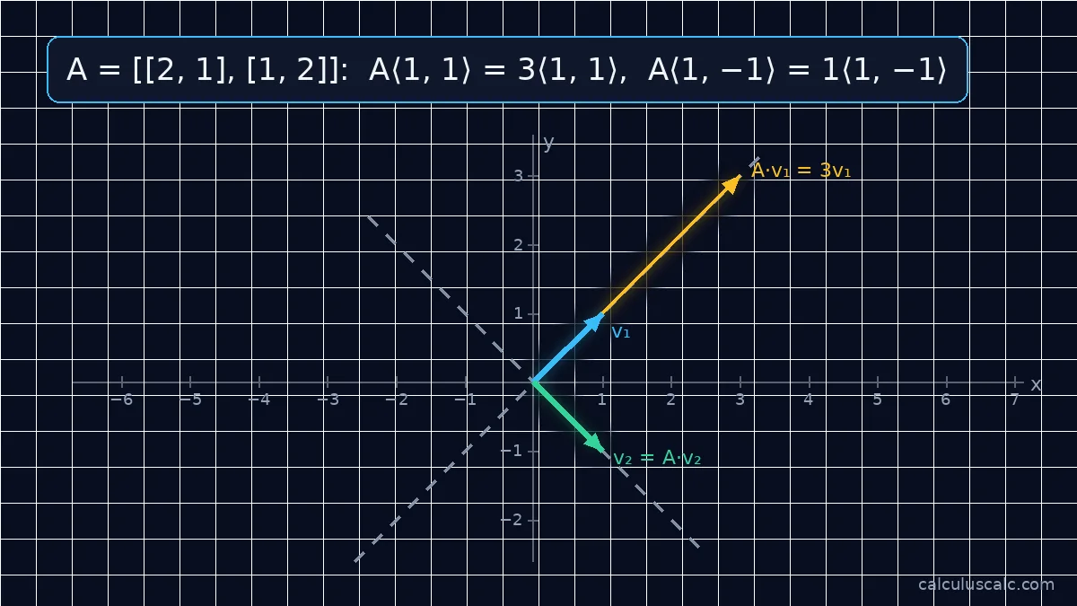
For ( A = begin{bmatrix} 2 & 1 1 & 2 end{bmatrix} ) (as loaded above):

$$detbegin{bmatrix} 2 - lambda & 1 1 & 2 - lambda end{bmatrix} = (2 - lambda)^2 - 1 = lambda^2 - 4lambda + 3 = (lambda - 1)(lambda - 3)$$

The eigenvalues are ( lambda_1 = 1 ) and ( lambda_2 = 3 ).

Eigenvector for ( lambda = 3 ): solve ( (A – 3I)v = 0 ), that is ( -x + y = 0 ), so ( v = langle 1, 1 rangle ). For ( lambda = 1 ): ( x + y = 0 ), so ( v = langle 1, -1 rangle ).

Check: ( Alangle 1, 1 rangle = langle 3, 3 rangle = 3langle 1, 1 rangle ). Any non-zero multiple of an eigenvector is also an eigenvector.

Worked example: a non-symmetric matrix

For ( A = begin{bmatrix} 4 & 1 2 & 3 end{bmatrix} ): trace 7, determinant 10, so ( lambda^2 – 7lambda + 10 = 0 ) and ( lambda = 2, 5 ). The eigenvectors are ( langle 1, -2 rangle ) for 2 and ( langle 1, 1 rangle ) for 5. You can verify these results using an eigenvalue calculator.

Worked example: complex eigenvalues

The rotation matrix ( begin{bmatrix} 0 & -1 1 & 0 end{bmatrix} ) has characteristic equation ( lambda^2 + 1 = 0 ), so ( lambda = pm i ). No real vector keeps its direction under a 90° rotation, which is exactly what complex eigenvalues signal. You can verify this with an eigenvalue calculator.

Worked example: a 3×3 matrix

For ( A = begin{bmatrix} 2 & 0 & 0 0 & 3 & 4 0 & 4 & 9 end{bmatrix} ), the characteristic equation is

$$lambda^3 - 14lambda^2 + 35lambda - 22 = 0$$

with roots ( lambda = 1, 2, 11 ). The eigenvectors are ( langle 0, 2, -1 rangle ), ( langle 1, 0, 0 rangle ) and ( langle 0, 1, 2 rangle ). Enter 2,0,0; 0,3,4; 0,4,9 to see the same result.

Useful checks

• The eigenvalues add up to the trace (the sum of the diagonal): ( 1 + 2 + 11 = 14 ).
• They multiply to the determinant: ( 1 cdot 2 cdot 11 = 22 ).
• A triangular matrix has its diagonal entries as eigenvalues.
• A real symmetric matrix always has real eigenvalues.

Repeated eigenvalues

When an eigenvalue repeats, it may have a whole plane of eigenvectors (as for the identity matrix) or just one direction (as for ( begin{bmatrix} 1 & 1 0 & 1 end{bmatrix} )). The calculator tells you which case you have.

Where eigenvalues are used

They solve systems of linear differential equations, find the principal axes of a shape, measure stability in physics and economics, rank web pages, and power principal component analysis in statistics.

Step-by-step method for a 2×2 matrix

1. Find the trace ( T = a + d ) and determinant ( D = ad – bc ) of ( begin{bmatrix} a & b c & d end{bmatrix} ).
2. Solve ( lambda^2 – Tlambda + D = 0 ) with the quadratic formula.
3. For each eigenvalue, write ( (A – lambda I)v = 0 ). The two equations are multiples of each other; therefore, solve either one for a non-zero v.
4. Check that ( Av = lambda v ).

Diagonalization and matrix powers

If A has n independent eigenvectors, then ( A = PDP^{-1} ), where the columns of P are the eigenvectors and D is the diagonal matrix of eigenvalues. Powers become easy: ( A^k = PD^kP^{-1} ). For ( A = begin{bmatrix} 2 & 1 1 & 2 end{bmatrix} ) with eigenvalues 1 and 3:

$$A^k = frac{1}{2}begin{bmatrix} 3^k + 1 & 3^k - 1 3^k - 1 & 3^k + 1 end{bmatrix}$$

For ( k = 2 ) this gives ( begin{bmatrix} 5 & 4 4 & 5 end{bmatrix} ), the same as multiplying A by itself (see matrix multiplication). For large k, the eigenvalue 3 dominates, which is the idea behind long-run behaviour in many models.

Worked example: a Markov chain

Each month 90% of a town’s customers stay with company X and 10% switch to Y. Conversely, Y keeps 50% and loses 50% to X. The transition matrix is ( begin{bmatrix} 0.9 & 0.5 0.1 & 0.5 end{bmatrix} ), with eigenvalues 1 and 0.4. The eigenvector for ( lambda = 1 ) is ( langle 5, 1 rangle ): in the long run X holds ( frac{5}{6} approx 83% ) of the market and Y ( frac{1}{6} ). Also, the eigenvalue 0.4 tells you how quickly the market settles: the gap shrinks by 60% each month.

Worked example: a system of differential equations

The system ( x’ = 2x + y, y’ = x + 2y ) has the matrix ( begin{bmatrix} 2 & 1 1 & 2 end{bmatrix} ). Its eigenvalues 1 and 3, with eigenvectors ( langle 1, -1 rangle ) and ( langle 1, 1 rangle ), give the general solution.

$$begin{bmatrix} x y end{bmatrix} = c_1 e^{t}begin{bmatrix} 1 -1 end{bmatrix} + c_2 e^{3t}begin{bmatrix} 1 1 end{bmatrix}$$

Positive eigenvalues mean solutions grow; however, negative ones mean they decay. See differential equations.

Practice problems

1. ( begin{bmatrix} 3 & 0 0 & -2 end{bmatrix} ).
2. ( begin{bmatrix} 1 & 2 2 & 1 end{bmatrix} ).
3. ( begin{bmatrix} 5 & 4 1 & 2 end{bmatrix} ).

Answers: 1. Diagonal, so 3 and −2, with eigenvectors ( langle 1, 0 rangle ) and ( langle 0, 1 rangle ). 2. Trace 2, determinant −3: ( lambda^2 – 2lambda – 3 = 0 ), so ( lambda = 3, -1 ), with eigenvectors ( langle 1, 1 rangle ) and ( langle 1, -1 rangle ). 3. Trace 7, determinant 6: ( lambda = 1, 6 ), with eigenvectors ( langle 1, -1 rangle ) and ( langle 4, 1 rangle ).

Related guides

• Matrix Multiplication
• Matrix Calculator
• Differential Equations
• Polynomials

Further reading

• Eigenvalues and eigenvectors (Wikipedia) — definitions, geometric meaning and applications.

FAQ

How do you find eigenvalues?

First, solve the characteristic equation ( det(A – lambda I) = 0 ). For a 2×2 matrix it is the quadratic ( lambda^2 – (text{trace})lambda + det A = 0 ).

How do you find an eigenvector?

For each eigenvalue, solve ( (A – lambda I)v = 0 ) for a non-zero v. Any non-zero multiple of a solution is also an eigenvector.

Can an eigenvalue be zero?

Yes. That happens exactly when the matrix is singular (its determinant is 0).

Can eigenvalues be complex?

Yes, for matrices like rotations. However, for real matrices they come in conjugate pairs ( a pm bi ).

What is the characteristic polynomial?

Also, ( det(A – lambda I) ) is a polynomial in λ whose roots are the eigenvalues. For an n×n matrix it has degree n.

Do eigenvectors have to be unit vectors?

No. Any non-zero multiple works. However, some textbooks normalize them to length 1, which you can do with the unit vector calculator.